What is a Covariance Matrix for Optimal Portfolio Allocation?
A simple explanation of the covariance matrix for portfolio allocation
👋 Hey there, Pedma here! Welcome to this free edition of Trading Research Hub’s Newsletter. Each week, I release a new research article with a trading strategy, its code, and much more.
Join over 5K+ traders and investors that read the newsletter!
As systematic or quantitative traders, we want to manage our risks, so that we can have better chances of achieving optimal returns for our portfolios.
And in order to manage our risks, we need to be aware of them in the first place.
A risk that we often encounter in our portfolios, is having a bunch of things, that are highly correlated with each other.
If every strategy or asset that we add to our portfolio is correlated, then we are increasing the risk, that when the market moves against us, the entire portfolio also goes in that direction.
If you’re looking for practical trading strategies, I write a weekly research series where we go through strategies, concepts, techniques, etc. Here’s my latest research article:
We can never truly eliminate the risk of correlations. Correlations change and break all the time. But at least we can get a bit smarter, on how we manage their risk during normal times.
Given this, what can be used as the mathematical representation, of the relationship between assets or strategies?
The covariance matrix.
Don’t worry, I will make this article as simple as possible to understand, because that’s how I learn also.
I don’t like complex academic jargon…
I think it doesn’t help and just makes people ever more confused that genuinely want to learn.
The covariance matrix basically helps in portfolio construction.
It is a mathematical representation of the covariances between multiple assets or strategies.
Covariance is a measure of how two things move together.
It provides us with information about the relationship between different assets or strategies.
We will also look into covariance and how it is calculated.
When the returns of two assets increase or decrease simultaneously, they have a positive covariance.
The opposite means that their covariance is negative.
This is important because we want to evaluate how to allocate between strategies given their diversifying factor.
If our goal is to minimize the impact of things that move together on our portfolio, we need to know those relationships, so that we can give different weights to things that affect our portfolio differently.
Today we will look into the details of how this covariance matrix gets calculated starting with the simplest concept of variance.
I’ve tried to make it as simple as possible, without diluting the importance of the content.
Let’s begin!
Index
Introduction
Index
What is Variance?
What is Covariance?
What is a Covariance Matrix?
Covariance Matrix in Finance
Conclusion
What is Variance?
Let’s understand the variance calculation first.
Variance is defined as the average of the squared differences from the mean.
It basically tells us how spread out the numbers in our data are.
In simple terms, imagine that the average yearly return of your model is 5%, and this year you only had 1% return.
The absolute difference is 4%.
The squared difference is 16%.
Now you may be wondering why do we square the differences?
When we square a number, the first thing it happens is that all negative differences are now positive.
Also any large deviations from the mean, get more weight, because we squared them.
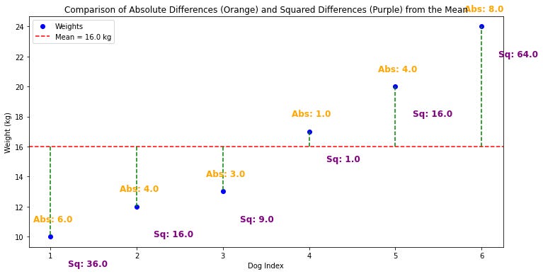
Look at the example above.
The absolute difference of the first value from the mean is only 6.
But the squared difference is 36.
Giving it more weight since it’s a larger deviation.
As the differences approach 0, their impact is smaller.
We want to give more impact to the points that are farther away from the mean, because outliers can significantly affect the overall distribution of the data.
By giving these “outliers” more weight, the variance provides us a better sense of how much the data spreads out, especially when there are only a few values that deviate greatly from the average.
In essence, squaring the differences ensures that the larger deviations will contribute disproportionately to the variance.
Also it reflects the true spread.
Had we only used the absolute differences, without squaring, all the differences would contribute equally to the measure of spread.
This will understate the true variability in the data, when some of the values are much further from the mean.
The formula for the variance is:
In a step-by-step process it looks like this:
Calculate the mean of the data set.
Subtract the mean from each data point, to find the deviation for each data point.
Square each deviation to eliminate negative values.
Sum all the squared deviations to get the total squared deviation.
Divide the sum, by the number of data points minus one, to find the sample variance.
import numpy as np

# Sample data
data = [10, 12, 8, 14, 13]  # Example data

# Step 1: Calculate the mean
mean = np.mean(data)

# Step 2: Subtract the mean from each data point and square the result
squared_deviations = [(x - mean) ** 2 for x in data]

# Step 3: Sum all the squared deviations
sum_of_squared_deviations = sum(squared_deviations)

# Step 4: Divide by the number of data points minus 1
sample_variance = sum_of_squared_deviations / (len(data) - 1)

print(f"Sample Variance: {sample_variance}")
What is Covariance?
Now that we understand variance, let’s look into what is covariance.
Imagine that you’re counting how many green apples are in five different grocery stores.
Variance, as we’ve discussed earlier, is calculated by first determining the average number of green apples across all stores.
Then, we measure how much the number of green apples, deviates from average in each store.
Finally, we square these deviations to emphasize larger differences.
This gives us a measure of how much the quantity of green apples varies from store to store.
Now also imagine that you count the red apples, in the same five stores.
Since the total number of red and green apples are from the same stores, we can pair them up, and look at their relationship.
Because we might be wondering:
“Do stores with a lot of green apples also have a lot of red apples?”
This is where covariance comes in.
It helps us understand if there’s a relationship between the counts of green and red apples.
How to calculate the covariance?
Here’s the formula:
Using our store example above, we do the following:
Calculate the difference between the number of green apples in store 1 and the average number of green apples across all stores.
Calculate the difference between the number of red apples in store 1 and the average number of red apples across all stores.
Multiply the differences obtained for green and red apples from store 1.
Repeat these steps for each subsequent store, calculating and multiplying the differences for each.
Sum all of the resulting products from each sample.
Finally, divide the total sum by the number of stores minus 1.
Now we can understand the relationship between two variables , and in our case, between the number of green and red apples across the store.
A positive covariance indicates that, stores with more green apples tend to have more red apples, and a negative covariance suggests the opposite.
import numpy as np

# Sample data for green and red apples
green_apples = [10, 12, 8, 14, 13]  # Example data for green apples
red_apples = [15, 18, 14, 20, 19]   # Example data for red apples

# Step 1: Calculate the means
mean_green = np.mean(green_apples)
mean_red = np.mean(red_apples)

# Step 2: Calculate differences from the mean for each sample and multiply them
products = [(green - mean_green) * (red - mean_red) for green, red in zip(green_apples, red_apples)]

# Step 3: Sum all of the values
sum_of_products = sum(products)

# Step 4: Divide by the number of samples minus 1
covariance = sum_of_products / (len(green_apples) - 1)

print(f"Covariance: {covariance}")
What is a Covariance Matrix?
Following our example above, now, imagine you have multiple types of apples:
Green
Red
Yellow
The covariance matrix is a tool that allows you to summarize all of these relationships in one place.
It’s a table that shows how each type of apple’s count, moves in relation to every other type.
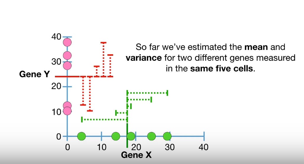
Here’s a good video explaining the covariance matrix:
In finance, the covariance matrix serves a similar purpose but on a much larger scale.
Instead of apples, you’re dealing with the returns of different assets or strategies in a portfolio.
For example in the video above, if we apply it to finance, the first chart measures the returns of Stock X, Stock Y and Stock Z, for year 1, 2, 3 and 4.
We will go more in-depth into an example for finance in the next chapter.
The covariance matrix provides a comprehensive view of how these assets move in relation to one another, which is essential for constructing a diversified portfolio that manages risk effectively.
Now let’s summarize the calculation for the Covariance Matrix:
Identify Variables and Calculate Averages:
Determine the variables (e.g., X, Y, Z).
Calculate the average (mean) for each variable.
Calculate Covariance for Each Pair:
For each pair of variables (e.g., X and Y):
Subtract the average of X from each X value, and the average of Y from each Y value.
Multiply these differences for each pair.
Sum all the products.
Divide by the number of data points to get the covariance.
Build the Covariance Matrix:
Place the covariance values in the matrix:
Covariances between different variables go in the off-diagonal positions.
Variances (covariances of a variable with itself) go on the diagonal.
Interpret the Matrix:
The diagonal shows the variances of each variable.
The off-diagonal shows the covariances between different variables.
And voilà.
You have your covariance matrix.
Let’s now look into it applied in the context of finance.
Covariance Matrix in Finance
Let’s consider a simple portfolio consisting of three assets: Stock A, Stock B, and Stock C. Here are the hypothetical monthly returns for each stock, over five months:
Stock A: [0.02, 0.03, 0.015, 0.05, 0.01]
Stock B: [0.01, 0.015, 0.02, 0.03, 0.025]
Stock C: [-0.01, 0.005, 0.015, 0.02, 0.01]
We can calculate the covariance matrix using these return values like this in python:
import numpy as np

# Monthly returns for each stock
returns_A = np.array([0.02, 0.03, 0.015, 0.05, 0.01])
returns_B = np.array([0.01, 0.015, 0.02, 0.03, 0.025])
returns_C = np.array([-0.01, 0.005, 0.015, 0.02, 0.01])

# Combine returns into a single matrix (each row is a different stock)
returns_matrix = np.array([returns_A, returns_B, returns_C])

# Calculate the covariance matrix
cov_matrix = np.cov(returns_matrix)

# Display the covariance matrix
print("Covariance Matrix:")
print(cov_matrix)Now let’s look into what the Values Represent
Diagonal Elements (Variance of Each Asset):
0.000301: This is the variance of Stock A's returns. Variance measures the volatility or risk of Stock A. A higher value indicates higher volatility.
0.000065: This is the variance of Stock B's returns, indicating that Stock B has lower volatility compared to Stock A.
0.000122: This is the variance of Stock C's returns, which is higher than Stock B's but lower than Stock A's, indicating moderate volatility.
Off-Diagonal Elements (Covariance Between Assets):
0.000205: This is the covariance between Stock A and Stock B. A positive value indicates that when Stock A’s returns increase, Stock B’s returns also tend to increase, and vice versa. The magnitude suggests the strength of this relationship.
0.000015: This is the covariance between Stock A and Stock C, a much smaller positive value, indicating a weaker positive relationship between these two stocks.
0.000020: This is the covariance between Stock B and Stock C, also a small positive value, indicating a weak positive relationship.
How to Use These Values for Portfolio Construction
Assessing Risk and Diversification:
Diversification: To reduce overall portfolio risk, you want to include assets that do not move together, i.e., have low or negative covariances. In this matrix, the covariances between stocks are all positive, but their magnitudes differ. Stocks with lower covariances (like Stock A and Stock C, with a covariance of 0.000015) are better candidates for diversification within the portfolio.
Volatility: Consider the variance values. Stocks with lower variances (like Stock B) will add stability to the portfolio, while stocks with higher variances (like Stock A) might increase potential returns but also add more risk.
Constructing the Portfolio:
Asset Weighting: If you're constructing a balanced portfolio, you might want to give more weight to assets with lower variances (e.g., Stock B) to reduce overall risk. However, depending on your risk tolerance, you might also want to include assets with higher variances (e.g., Stock A) to potentially increase returns.
Correlation Consideration: While all the stocks in this example have positive covariances, which suggest they generally move in the same direction, the lower covariance values indicate weaker correlations. This information can guide you in pairing assets in the portfolio to achieve a good mix of risk and return.
Optimization:
Mean-Variance Optimization: Using the covariance matrix in conjunction with expected returns, you can apply mean-variance optimization to find the portfolio with the maximum expected return for a given level of risk. This is the basis of Modern Portfolio Theory (MPT), where you aim to construct a portfolio that lies on the efficient frontier.
Example Actionable Strategy
Moderate Risk Portfolio: Suppose you want to construct a portfolio that balances risk and returns. You might allocate more weight to Stock B (lower variance, lower risk) and Stock C (moderate variance, low covariance with others) to keep the portfolio stable. Stock A could be included but with a smaller allocation due to its higher variance.
Aggressive Portfolio: If you're seeking higher returns and are willing to accept more risk, you might allocate more weight to Stock A, despite its higher variance, because it could potentially offer higher returns. However, to maintain some diversification, you would still include Stocks B and C, with careful consideration of their covariances.
Conclusion
The covariance matrix is not just a theoretical concept but a practical tool that plays a very important role in modern portfolio management.
By capturing the relationships between different assets or strategies, the covariance matrix allows the investor, to understand better their portfolio in terms of risk and diversification.
For example in our example above, we analyzed how Stock A, Stock B and Stock C’s variances highlight the individual risks of the assets or strategies, and how these interact.
It offers insights into both the individual volatility of the assets and the relationships between these assets.
If we study and carefully interpret the information, we can create portfolios that are better diversified, more aligned with our risk tolerance, and optimized for potential returns.
In the next article, we will put together strategies, and find out how we can optimally allocate between them, given their diversification factors.
I hope you’ve enjoyed today’s article!
If you want to have my own custom assistance, with your systematic trading business, I help individuals and enterprises, implement and deploy strategy portfolios, tailored to their specific needs.
If you want to discuss the possibility of working with me:
Disclaimer: The content and information provided by the Trading Research Hub, including all other materials, are for educational and informational purposes only and should not be considered financial advice or a recommendation to buy or sell any type of security or investment. Always conduct your own research and consult with a licensed financial professional before making any investment decisions. Trading and investing can involve significant risk of loss, and you should understand these risks before making any financial decisions.


